Intro to Python Image Processing in Computational Photography

前言

原文：Intro to Python Image Processing in Computational Photography **作者：RADU BALABAN **

正文

Computational photography is about enhancing the photographic process with computation. While we normally tend to think that this applies only to post-processing the end result (similar to photo editing), the possibilities are much richer since computation can be enabled at every step of the photographic process—starting with the scene illumination, continuing with the lens, and eventually even at the display of the captured image. This is important because it allows for doing much more and in different ways than what can be achieved with a normal camera. It is also important because the most prevalent type of camera nowadays—the mobile camera—is not particularly powerful compared to its larger sibling (the DSLR), yet it manages to do a good job by harnessing the computing power it has available on the device. We’ll take a look at two examples where computation can enhance photography—more precisely, we’ll see how simply taking more shots and using a bit of Python to combine them can create nice results in two situations where mobile camera hardware doesn’t really shine—low light and high dynamic range.

Low-light Photography

Let’s say we want to take a low-light photograph of a scene, but the camera has a small aperture (lens) and limited exposure time. This a typical situation for mobile phone cameras which, given a low light scene, could produce an image like this (taken with an iPhone 6 camera): 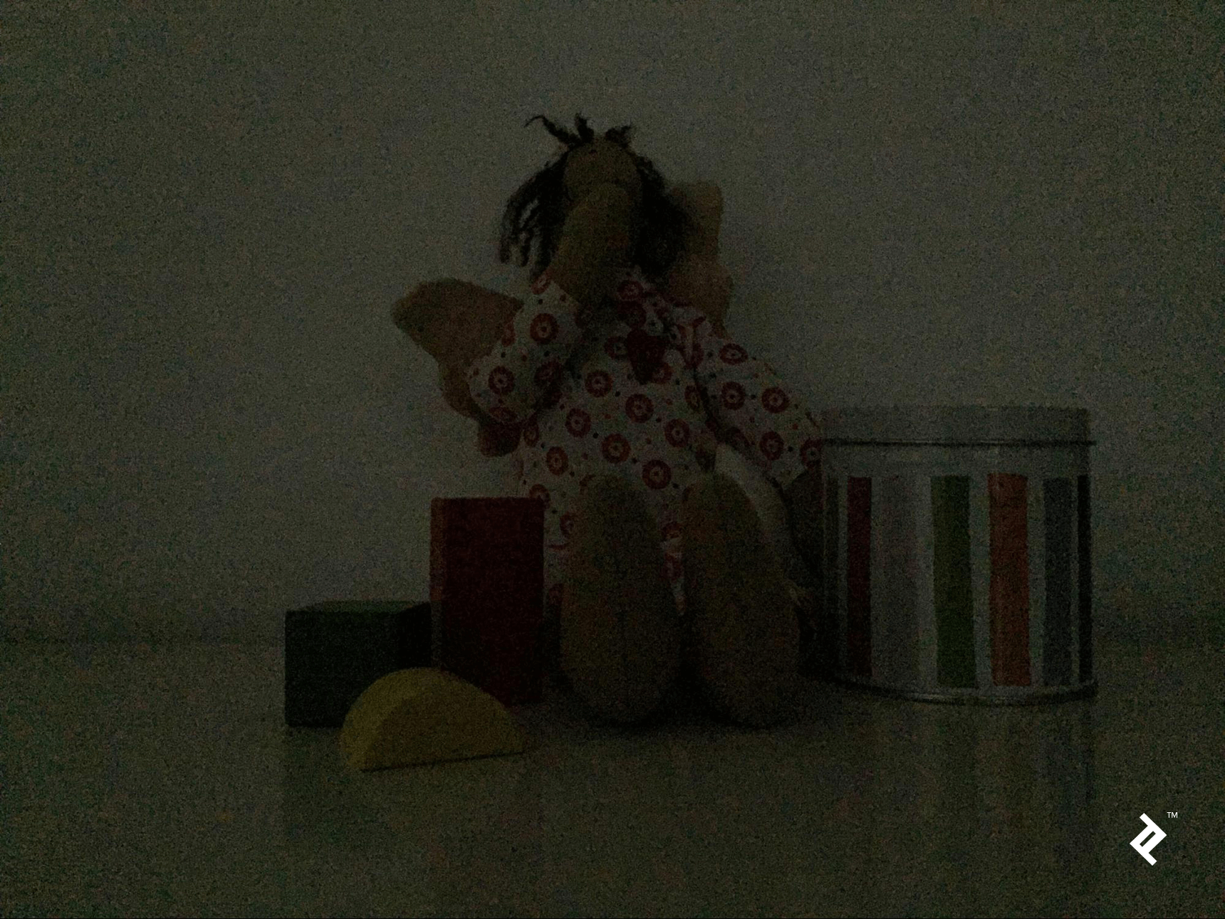If we try to improve the contrast the result is the following, which is also quite bad: 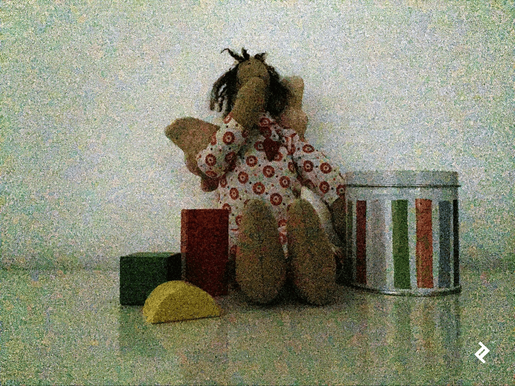What happens? Where does all this noise come from? The answer is that the noise comes from the sensor—the device that tries to determine when the light strikes it and how intense that light is. In low light, however, it has to increase its sensitivity by a great deal to register anything, and that high sensitivity means it also starts detecting false positives—photons that simply aren’t there. (As a side note, this problem does not affect only devices, but also us humans: Next time you’re in a dark room, take a moment to notice the noise present in your visual field.) Some amount of noise will always be present in an imaging device; however, if the signal (useful information) has high intensity, the noise will be negligible (high signal to noise ratio). When the signal is low—such as in low light—the noise will stand out (low signal to noise). Still, we can overcome the noise problem, even with all the camera limitations, in order to get better shots than the one above. To do that, we need take into account what happens over time: The signal will remain the same (same scene and we assume it’s static) while the noise will be completely random. This means that, if we take many shots of the scene, they will have different versions of the noise, but the same useful information. So, if we average many images taken over time, the noise will cancel out while the signal will be unaffected. The following illustration shows a simplified example: We have a signal (triangle) affected by noise, and we try to recover the signal by averaging multiple instances of the same signal affected by different noise. 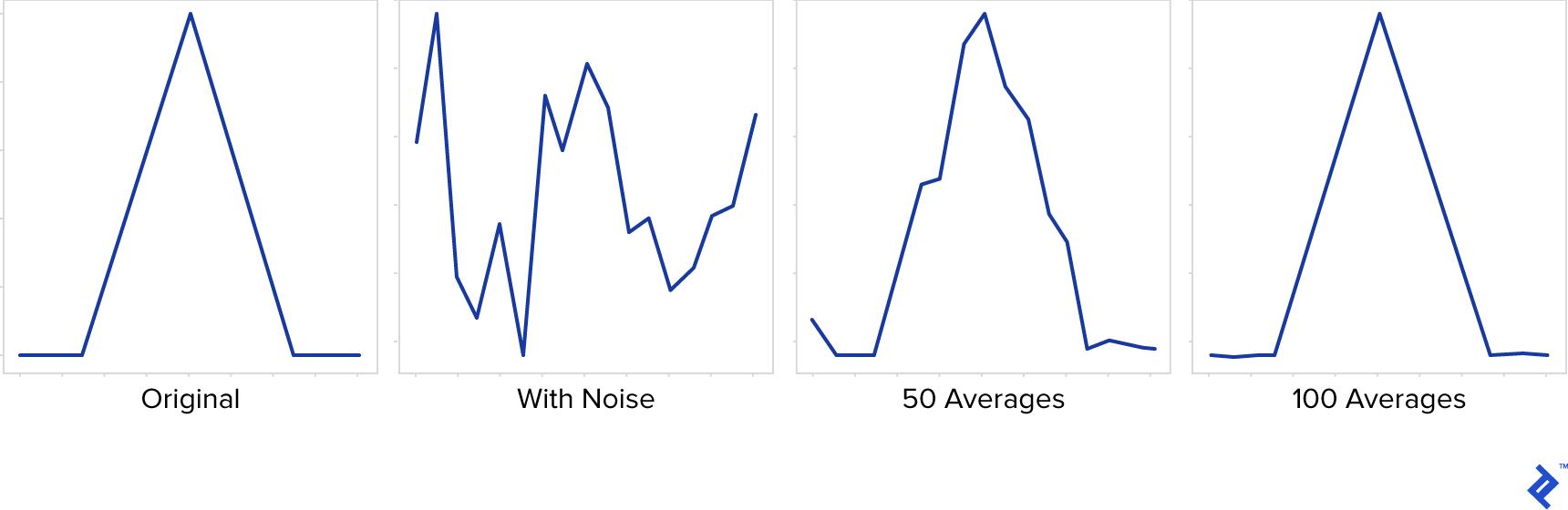We see that, although the noise is strong enough to completely distort the signal in any single instance, averaging progressively reduces the noise and we recover the original signal. Let’s see how this principle applies to images: First, we need to take multiple shots of the subject with the maximum exposure that the camera allows. For best results, use an app that allows manual shooting. It is important that the shots are taken from the same location, so a (improvised) tripod will help. More shots will generally mean better quality, but the exact number depends on the situation: how much light there is, how sensitive the camera is, etc. A good range could be anywhere between 10 and 100. Once we have these images (in raw format if possible), we can read and process them in Python. For those not familiar to image processing in Python, we should mention that an image is represented as a 2D array of byte values (0-255)—that is, for a monochrome or grayscale image. A color image can be thought of as a set of three such images, one for each color channel (R, G, B), or effectively a 3D array indexed by vertical position, horizontal position and color channel (0, 1, 2). We will make use of two libraries: NumPy (http://www.numpy.org/) and OpenCV (https://opencv.org/). The first allows us to perform computations on arrays very effectively (with surprisingly short code), while OpenCV handles reading/writing of the image files in this case, but is a lot more capable, providing many advanced graphics procedures—some of which we will use later in the article.

import os
import numpy as np
import cv2

folder = 'source_folder'

# We get all the image files from the source folder
files = list([os.path.join(folder, f) for f in os.listdir(folder)])

# We compute the average by adding up the images
# Start from an explicitly set as floating point, in order to force the
# conversion of the 8-bit values from the images, which would otherwise overflow
average = cv2.imread(files[0]).astype(np.float)
for file in files[1:]:
    image = cv2.imread(file)
    # NumPy adds two images element wise, so pixel by pixel / channel by channel
    average += image
 
# Divide by count (again each pixel/channel is divided)
average /= len(files)

# Normalize the image, to spread the pixel intensities across 0..255
# This will brighten the image without losing information
output = cv2.normalize(average, None, 0, 255, cv2.NORM_MINMAX)

# Save the output
cv2.imwrite('output.png', output)

The result (with auto-contrast applied) shows that the noise is gone, a very large improvement from the original image. 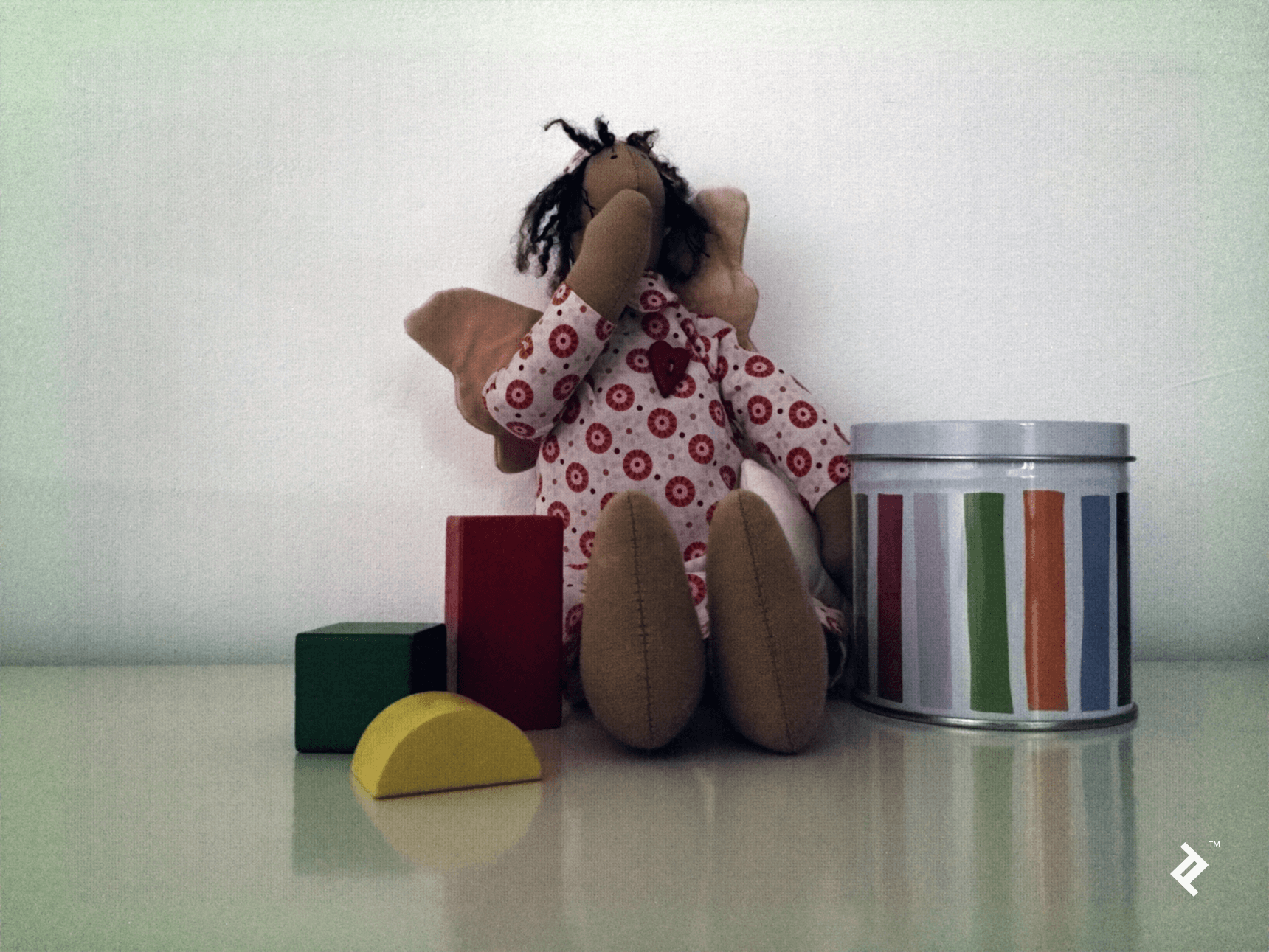However, we still notice some strange artifacts, such as the greenish frame and the gridlike pattern. This time, it’s not a random noise, but a fixed pattern noise. What happened?

A close-up of the top left corner, showing the green frame and grid pattern

Again, we can blame it on the sensor. In this case, we see that different parts of the sensor react differently to light, resulting in a visible pattern. Some elements of these patterns are regular and are most probably related to the sensor substrate (metal/silicon) and how it reflects/absorbs incoming photons. Other elements, such as the white pixel, are simply defective sensor pixels, which can be overly sensitive or overly insensitive to light. Fortunately, there is a way to get rid of this type of noise too. It is called dark frame subtraction. To do that, we need an image of the pattern noise itself, and this can be obtained if we photograph darkness. Yes, that’s right—just cover the camera hole and take a lot of pictures (say 100) with maximum exposure time and ISO value, and process them as described above. When averaging over many black frames (which are not in fact black, due to the random noise) we will end up with the fixed pattern noise. We can assume this fixed noise will stay constant, so this step is only needed once: The resulting image can be reused for all future low-light shots. Here is how the top right part of the pattern noise (contrast adjusted) looks like for an iPhone 6: 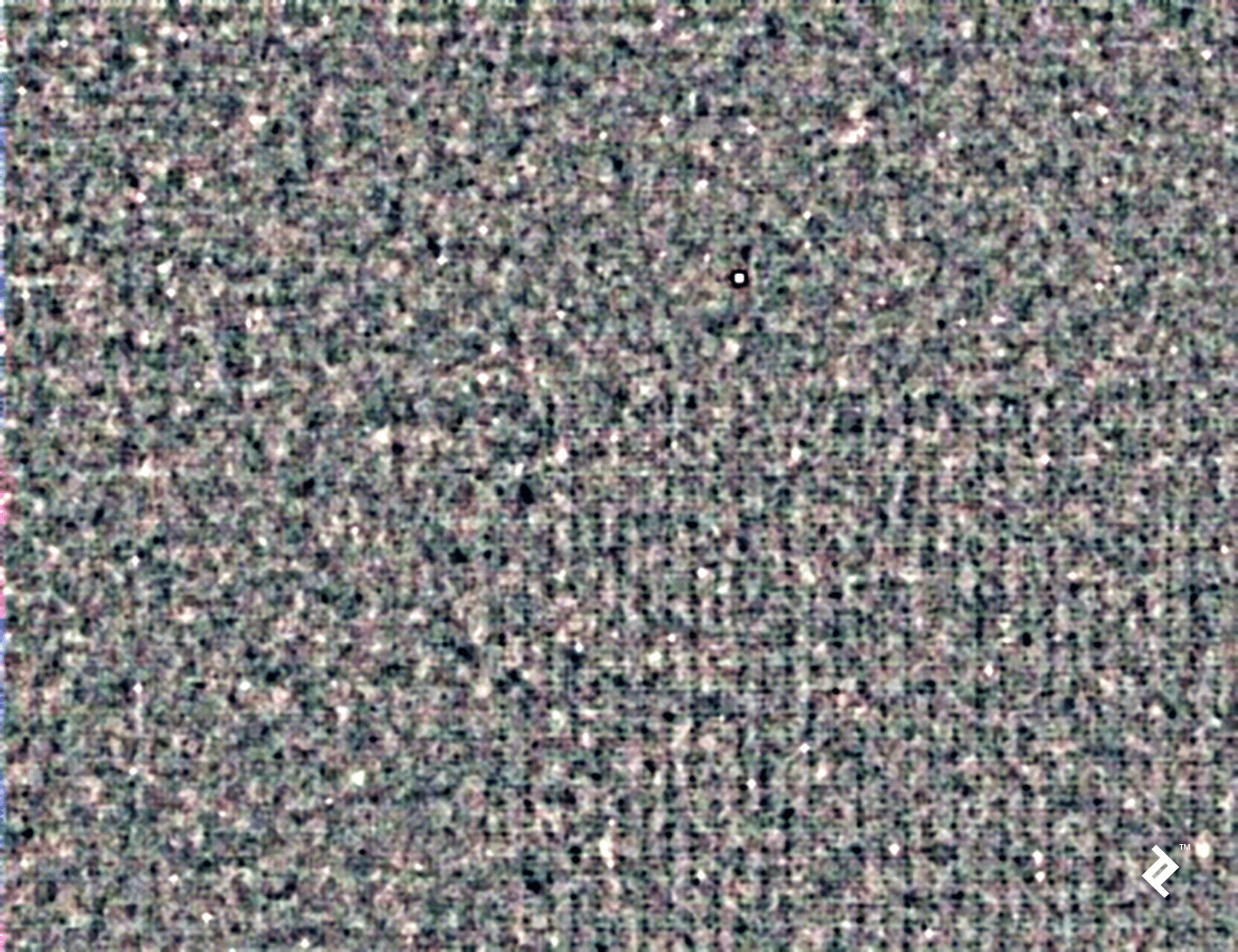Again, we notice the grid-like texture, and even what appears to be a stuck white pixel. Once we have the value of this dark frame noise (in the average_noise variable), we can simply subtract it from our shot so far, before normalizing:

average -= average_noise

output = cv2.normalize(average, None, 0, 255, cv2.NORM_MINMAX)
cv2.imwrite('output.png', output)

Here is our final photo: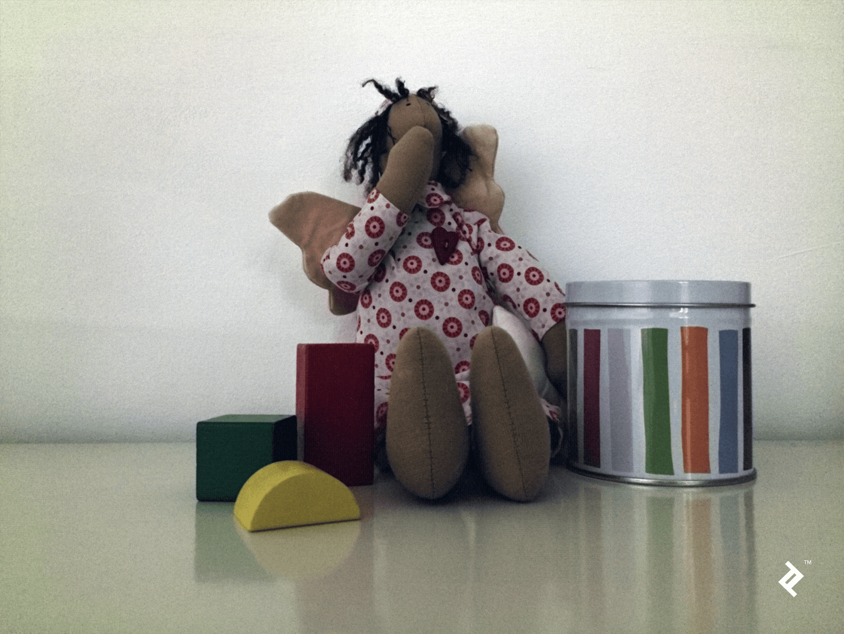

High Dynamic Range

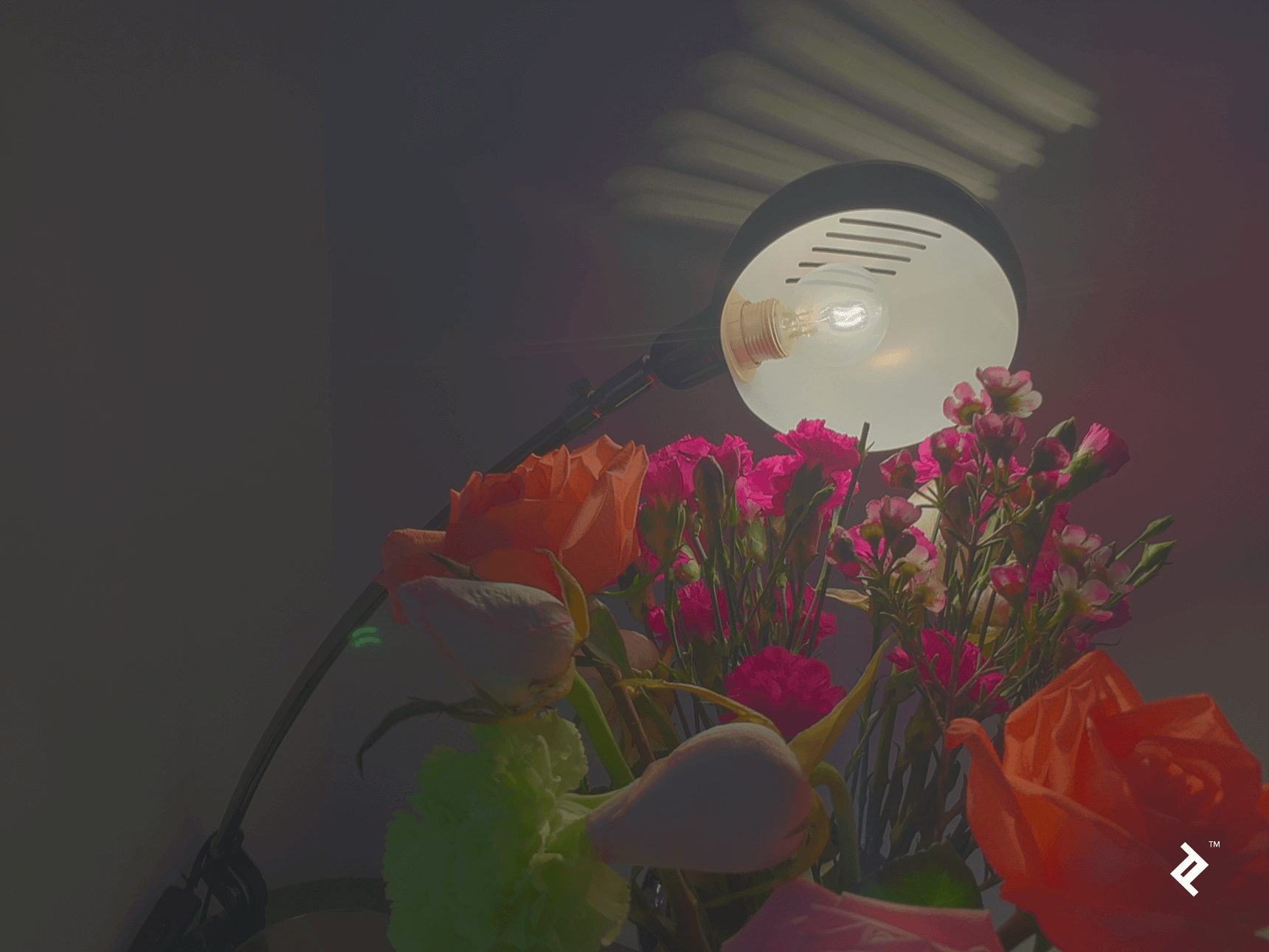
Another limitation that a small (mobile) camera has is its small dynamic range, meaning the range of light intensities at which it can capture details is rather small. In other words, the camera is able to capture only a narrow band of the light intensities from a scene; the intensities below that band appear as pure black, while the intensities above it appear as pure white, and any details are lost from those regions. However, there is a trick that the camera (or photographer) can use—and that is adjusting the exposure time (the time the sensor is exposed to the light) in order to control the total amount of light that gets to the sensor, effectively shifting the range up or down in order to capture the most appropriate range for a given scene. But this is a compromise. Many details fail to make it into the final photo. In the two images below, we see the same scene captured with different exposure times: a very short exposure (1/1000 sec), a medium exposure (1/50 sec) and a long exposure (1/4 sec). 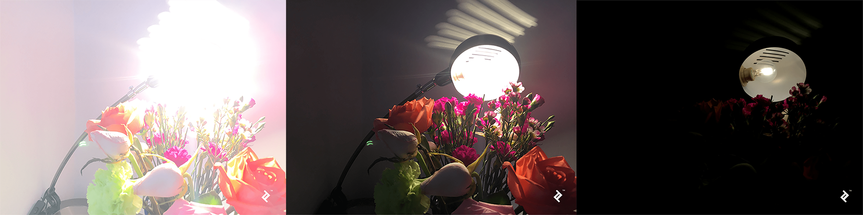As you can see, neither of the three images is able to capture all the available details: The filament of the lamp is visible only in the first shot, and some of the flower details are visible either in the middle or the last shot but not both. The good news is that there’s is something we can do about it, and again it involves building on multiple shots with a bit of Python code. The approach we’ll take is based on the work of Paul Debevec et al., who describes the method in his paper here. The method works like this: First, it requires multiple shots of the same scene (stationary) but with different exposure times. Again, as in the previous case, we need a tripod or support to make sure the camera does not move at all. We also need a manual shooting app (if using a phone) so that we can control the exposure time and prevent camera auto-adjustments. The number of shots required depends on the range of intensities present in the image (from three upwards), and the exposure times should be spaced across that range so that the details we are interested in preserving show up clearly in at least one shot. Next, an algorithm is used to reconstruct the response curve of the camera based on the color of the same pixels across the different exposure times. This basically lets us establish a map between the real scene brightness of a point, the exposure time, and the value that the corresponding pixel will have in the captured image. We will use the implementation of Debevec’s method from the OpenCV library.

# Read all the files with OpenCV
files = ['1.jpg', '2.jpg', '3.jpg', '4.jpg', '5.jpg']
images = list([cv2.imread(f) for f in files])
# Compute the exposure times in seconds
exposures = np.float32([1. / t for t in [1000, 500, 100, 50, 10]])

# Compute the response curve
calibration = cv2.createCalibrateDebevec()
response = calibration.process(images, exposures)

The response curve looks something like this: 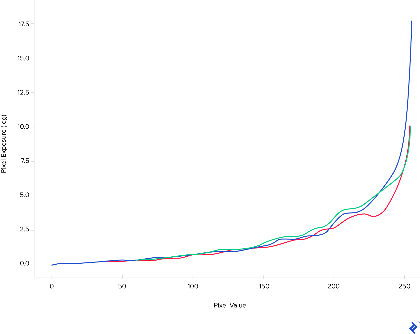On the vertical axis, we have the cumulative effect of the scene brightness of a point and the exposure time, while on the horizontal axis we have the value (0 to 255 per channel) the corresponding pixel will have. This curve than allows us to perform the reverse operation (which is the next step in the process)—given the pixel value and the exposure time, we can compute the real brightness of each point in the scene. This brightness value is called irradiance, and it measures the amount of light energy that falls on a unit of sensor area. Unlike the image data, it is represented using floating point numbers because it reflects a much wider range of values (hence, high dynamic range). Once we have the irradiance image (the HDR image) we can simply save it:

# Compute the HDR image
merge = cv2.createMergeDebevec()
hdr = merge.process(images, exposures, response)

# Save it to disk
cv2.imwrite('hdr_image.hdr', hdr)

For those of us lucky enough to have an HDR display (which is getting more and more common), it may be possible to visualize this image directly in all its glory. Unfortunately, the HDR standards are still in their infancy, so the process to do that may be somewhat different for different displays. For the rest of us, the good news is that we can still take advantage of this data, although a normal display requires the image to have byte value (0-255) channels. While we need to give up some of the richness of the irradiance map, at least we have the control over how to do it. This process is called tone-mapping and it involves converting the floating point irradiance map (with a high range of values) to a standard byte value image. There are techniques to do that so that many of the extra details are preserved. Just to give you an example of how this can work, imagine that before we squeeze the floating point range into byte values, we enhance (sharpen) the edges that are present in the HDR image. Enhancing these edges will help preserve them (and implicitly the detail they provide) also in the low dynamic range image. OpenCV provides a set of these tone-mapping operators, such as Drago, Durand, Mantiuk or Reinhardt. Here is an example of how one of these operators (Durand) can be used and of the result it produces.

durand = cv2.createTonemapDurand(gamma=2.5)
ldr = durand.process(hdr)

# Tonemap operators create floating point images with values in the 0..1 range
# This is why we multiply the image with 255 before saving
cv2.imwrite('durand_image.png', ldr * 255)

Using Python, you can also create your own operators if you need more control over the process. For instance, this is the result obtained with a custom operator that removes intensities that are represented in very few pixels before shrinking the value range to 8 bits (followed by an auto-contrast step): 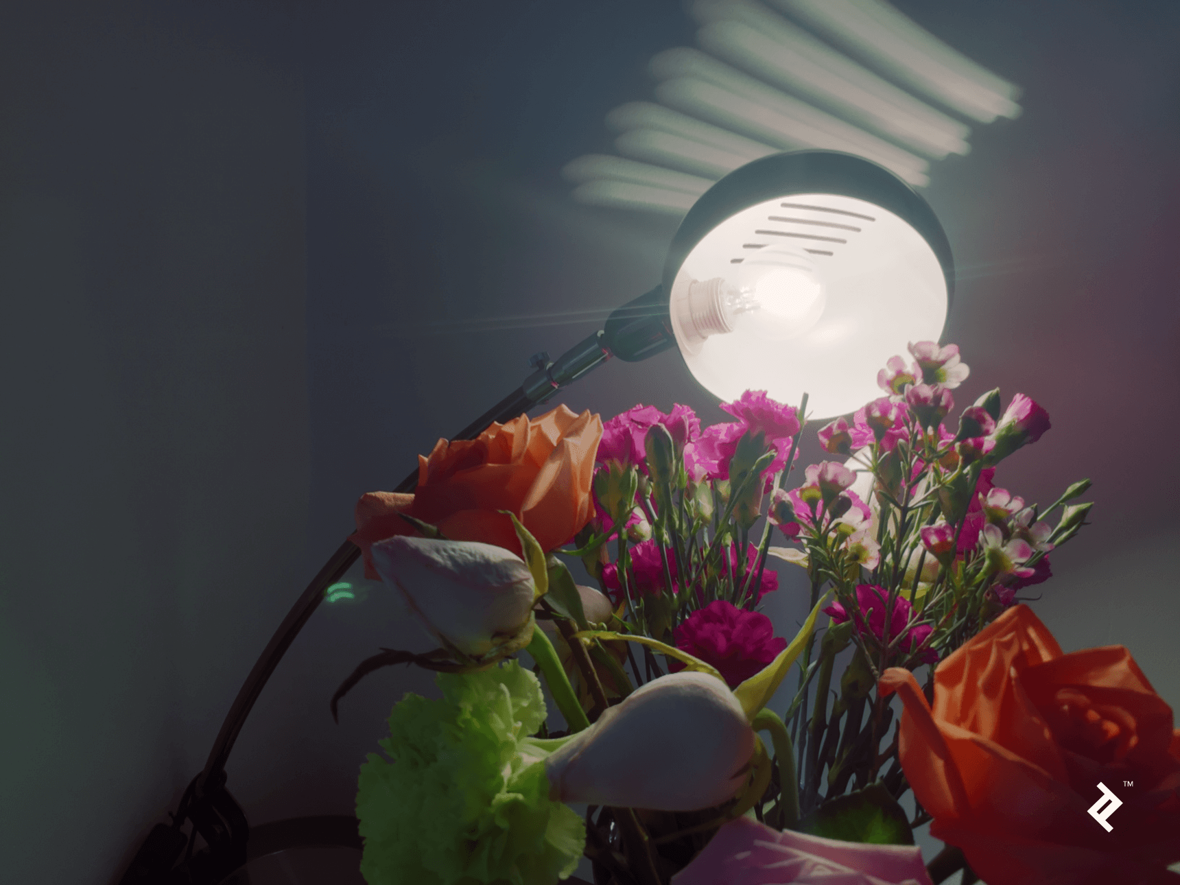And here is the code for the above operator:

def countTonemap(hdr, min_fraction=0.0005):
	counts, ranges = np.histogram(hdr, 256)
	min_count = min_fraction * hdr.size
	delta_range = ranges[1] - ranges[0]

	image = hdr.copy()
	for i in range(len(counts)):
    	if counts[i] < min_count:
        	image[image >= ranges[i + 1]] -= delta_range
        	ranges -= delta_range

	return cv2.normalize(image, None, 0, 1, cv2.NORM_MINMAX)

Conclusion

We’ve seen how with a bit of Python and a couple supporting libraries, we can push the limits of the physical camera in order to improve the end result. Both examples we’ve discussed use multiple low-quality shots to create something better, but there are many other approaches for different problems and limitations. While many camera phones have store or built-in apps that address these particular examples, it is clearly not difficult at all to program these by hand and to enjoy the higher level of control and understanding that can be gained. If you’re interested in image computations on a mobile device, check out OpenCV Tutorial: Real-time Object Detection Using MSER in iOS by fellow Toptaler and elite OpenCV developer Altaibayar Tseveenbayar.

UNDERSTANDING THE BASICS

How does the sensor in a camera work?

The sensor translates the incoming light into electrical signals, which are then amplified and digitized. Its surface is divided into pixels, which are further divided into channels. Therefore, the sensor produces three numbers corresponding to red, green and blue light intensities for every point in the scene.

What is the meaning of image processing?

Image processing refers to any computational steps taken after a raw image has been captured by the sensor, in order to either enhance or modify it.

How does image processing work?

Image processing is done in software by applying numerical operations on the image data. Most common image processing techniques have a solid mathematical background.

What is Python, NumPy and OpenCV?

Python is a programming language well suited for scientific computing. NumPy is a Python library that simplifies doing numerical operations on arrays. OpenCV is a specialized library, focused on image processing and computer vision.

Why are very low-light photographs noisy?

In low light and with limited exposure, there is a very small amount of light energy that falls on the sensor. The sensor tries to compensate by amplifying the signal, but ends up also amplifying its own electrical noise.

What is HDR photography?

High dynamic range (HDR) photography refers to capturing more accurately the physical light intensity in a scene. Conventional digital photography uses only a small number of intensity levels (typically 256).

What is tone mapping?

Tone mapping is the technique that transforms an HDR image into a conventional image, preserving most details so that the image can be shown on a non-HDR display.